The map is not the model

—

Most real estate mistakes are local mistakes wearing institutional clothes.

The model says the submarket is growing. The broker deck says the median household income is high. The investment memo says the site sits inside the path of growth. All three statements can be true and still miss the actual question: growth where, measured how, and close enough to matter?

That is why I like H3.

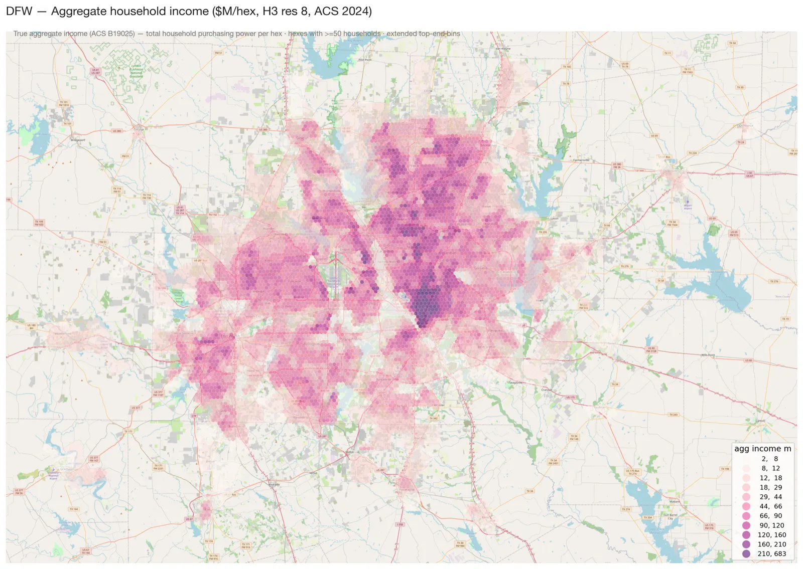
H3 is a global hexagonal grid system. It takes the earth and divides it into consistently sized cells. (It’s one of several — S2, geohash, and quad-tree systems do similar work; hexes win on uniform neighbor distance and good open tooling, and for most CRE applications the choice rarely changes the conclusion.) At resolution 8, the DFW map above is cut into hexes of roughly 182 acres each. At resolution 9, the cells are about 26 acres. At resolution 10, about 3.7 acres. That means you can put different kinds of data into the same spatial accounting unit: households, income, jobs, parcels, appraised value, traffic counts, leases, rent comps, permits, crime, schools, drive times, and store locations.

For a layperson, that sounds like a prettier map.

For an investor, it is more useful than that. It is a way to turn geography into an auditable underwriting surface. Auditable means: if a sponsor says trade-area income grew 22% from 2016 to 2024, an LP (or a fund’s strategy team, or an outside consultant) can recompute the same metric on the same hex grid using public ACS data and check whether it lines up. The number either matches or it doesn’t. The submarket label doesn’t get to define itself.

The map above shows aggregate household income across DFW, measured in dollars per H3 cell. Not median income. Aggregate income. That distinction matters. Median income tells you the typical household’s income. Aggregate income tells you the total household purchasing power sitting in that small patch of ground. A wealthy exurban pocket with 80 households can have a very high median income and a low aggregate-income base. A denser middle-income corridor can have lower median income and far more total spending power.

For site selection, the second number is often the one that pays rent — for grocery-anchored retail, necessity retail, multifamily, and most QSR. A luxury concept goes the other way: it wants the concentration of high-income households, not the aggregate, because aggregate income mass that comes from middle-income density doesn’t show up at the register. Different assets read different surfaces.

Here is the same DFW grid showing a different one — the share of households in each hex reporting investment income (interest, dividends, or net rental income) on their tax returns:

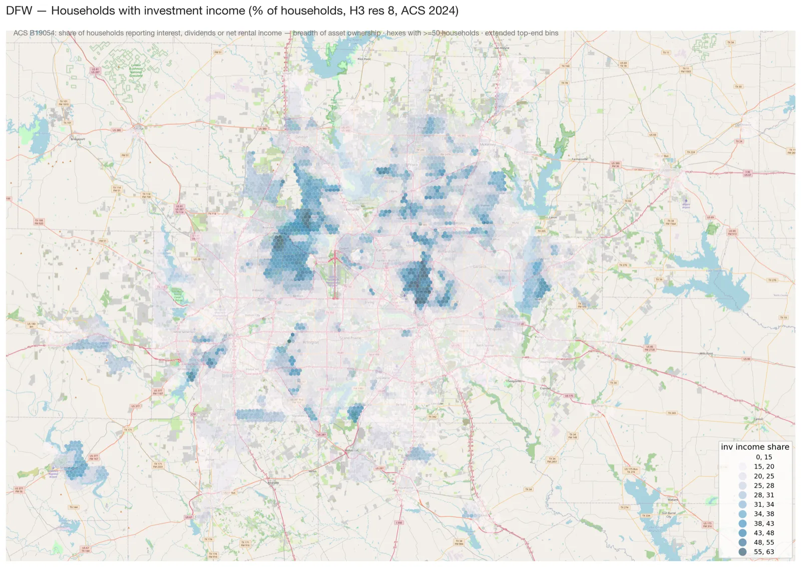
This is a breadth-of-asset-ownership map, not a dollar-mass map. The median DFW hex has about 15 percent of households pulling some recurring income from a balance sheet rather than from a paycheck; the top hexes run above 60 percent. The pattern does not match the aggregate-income map above. Aggregate income peaks where the high-earnings corridors cluster — Plano, Frisco, the Tollway. Investment income share peaks in older-wealth submarkets — the Park Cities, Preston Hollow, parts of Westover Hills in Fort Worth — places where the median household earns less than the very top earners but holds substantially more of its prosperity in already-accumulated assets.

The distinction is the one most submarket conversations skip past. A grocery-anchored center reads the first map. A private bank, an estate-planning firm, a wealth manager’s branch, or a luxury concept that lives on discretionary spending out of existing wealth reads the second. The two surfaces overlap at the edges and diverge in the middle, and which one a tenant should be reading depends on what’s actually on the menu — not on the submarket label. The same is true for the LP underwriting the building they sit in.

Why this matters to LPs

LPs do not usually lose money because they lack maps. They lose money because the map in the memo is not connected tightly enough to the actual investment question.

If the question is “Can this grocery-anchored center support a stronger tenant mix?”, you need household income mass, drive-time access, leakage, and competing centers. If the question is “Can this industrial site lease to regional distribution users?”, you need labor, highway access, truck routes, airport and intermodal access, and land basis. If the question is “Is this multifamily site in the path of growth?”, you need population growth, household formation, income growth, rent growth, supply pipeline, and commute gravity.

Those are different questions. A single submarket label answers none of them.

H3 helps because it forces the underwriter to separate the question from the boundary. ZIP codes are postal tools. Census tracts are statistical tools. City limits are political tools. Counties are administrative tools. None of those boundaries were designed to answer whether a particular parcel at a particular basis should receive capital.

Hexes are not a cure-all either. They are just less interested in our old categories.

The useful move is this: put the asset, its competitors, its customers, and its constraints onto the same grid. Then ask whether the local pattern supports the business plan.

That is the difference between “Dallas is growing” and “this site sits on the wrong side of the demand surface.”

What the DFW map is really showing

DFW is the right example because it is not one market.

It is Dallas, Fort Worth, Las Colinas, Plano, Frisco, Alliance, and the Tollway corridor — plus a growing set of outer nodes that are not waiting for downtown Dallas to bless them. The metro is polycentric; it has multiple centers of gravity.

On the aggregate-income map, the obvious story is the northern arc: Plano, Frisco, McKinney, Allen, Prosper, and the Tollway corridor. But the more important investment point is not that North Dallas is affluent. That is table stakes. The useful point is that income mass does not move as a smooth circle outward from downtown. It forms corridors, ridges, gaps, and secondary basins.

That matters because CRE cash flows are local. A tenant does not lease “DFW.” A resident does not commute from “the metro.” A retailer does not pull customers from a county label. The trade area is a geometry problem before it is a spreadsheet problem.

An LP looking at a deal in this region should want to know where the site sits relative to three surfaces:

• Demand mass: households, income, and spending power within the relevant catchment.
• Economic gravity: jobs, workers, commute corridors, and daytime population.
• Competitive supply: existing assets, planned supply, land availability, and achievable basis.

H3 does not answer the investment question by itself. It lets you ask the same question repeatedly across sites without changing the ruler.

That is underrated. A consistent ruler is how you notice when a sponsor is quietly changing the argument from one deal to the next.

Here is economic gravity for the same DFW — jobs density today, and where jobs grew or thinned over the last decade:

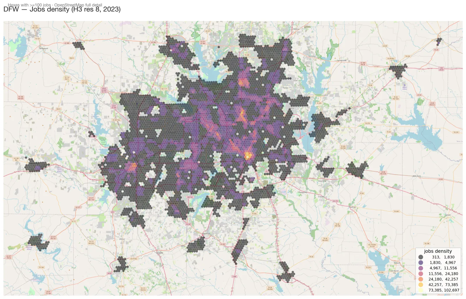
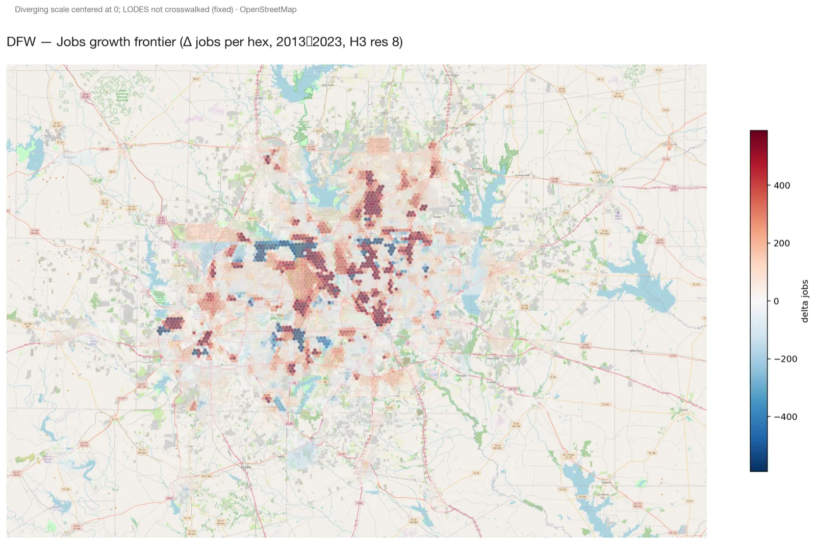
Density tells you where the workers go now. Growth tells you whether the gravity is concentrating or relaxing — and where. The two maps together, on the same hex grid as the income map above, make the structural question visible: the demand corridors on the income map and the gravity corridors on these maps are not the same shape. A multifamily LP needs to know which one their sponsor is selling. An industrial LP needs to know which one their tenant is hiring against. The submarket label answers neither.

The resolution is an underwriting choice

The first way people misuse H3 is by choosing a resolution because the map looks good.

Resolution is not an aesthetic decision. It is an underwriting decision.

At DFW scale, resolution 8 works well for a metro overview. Each cell is roughly 182 acres. That is small enough to show corridors and neighborhood-level variation, but large enough that the map does not turn into confetti. For a county or suburban trade-area screen, resolution 9 is often better: about 26 acres per cell. For parcel-adjacent fiscal productivity or downtown block analysis, resolution 10 can work: about 3.7 acres per cell.

But smaller is not always better. Smaller cells create more apparent precision. Apparent precision is dangerous because it feels like diligence.

If the underlying source is ACS 5-year data at the census tract level, slicing it into tiny hexes does not create block-level truth. It creates a finer allocation of tract-level estimates. The cell got smaller; the evidence did not necessarily get better.

This is the modifiable areal unit problem in plain English: any aggregation boundary, including a hex, shapes the pattern you see. A 182-acre hex still averages out internal variance, just less than a 2,000-acre tract does. H3 does not escape this. It gives you a consistent ruler so the distortion is the same across sites — which is the part that matters for cross-site comparison.

That is the practitioner rule: match the H3 resolution to the resolution of the decision and the source data.

Use res 8 for metro pattern recognition. Use res 9 for site-area screening. Use res 10 when you have parcel, point, or high-confidence local data. Do not use res 10 just because the map looks more impressive in an investment committee deck. The map will not be the one making capital calls in five years.

Time series are where this gets serious

A static map is useful. A time series is more useful and more dangerous.

Suppose you want to compare household income around a DFW site in 2011, 2016, and 2024. The easy version is to pull ACS data for each year, map it, and show the color getting darker. That is also the version most likely to lie to you.

There are three reasons.

First, the Census redraws tract boundaries — but not continuously. Tract geographies change on the decennial census (2000, 2010, 2020, 2030). A time series that spans one of those years crosses a discrete boundary change; a comparison entirely inside a decade does not. The 2011-to-2024 comparison above crosses two such changes (2010 and 2020 vintages); 2016-to-2024 crosses one (2020). A tract in the 2010 geography may split, merge, or change shape in 2020, and comparing the old tract directly to the new tract can mean comparing different pieces of land and calling it growth.

Second, income must be deflated. A dollar in 2011 is not a dollar in 2024. Nominal income growth can look like local prosperity when part of it is just inflation.

Third, ACS estimates have noise. The ACS is a survey, not a full count. Small geographies can carry large margins of error, especially when you are slicing into income bands, rent bands, or subpopulations.

This is where the census crosswalk matters. A crosswalk translates older tract data into newer geography — if a 2011 tract was later split into three 2020 tracts, the crosswalk allocates the old population, households, or income onto the new boundaries, weighted by land area, population, or housing units depending on the variable. The translation is not perfect. It is better than pretending the boundaries never changed.

For CRE, the crosswalk is not a technical nicety. It is the difference between underwriting real growth and underwriting a cartographic artifact.

If a sponsor says a trade area grew 40 percent over a decade, I want to know whether the analysis held the geography constant. If it did not, the first question is not whether the growth is impressive. The first question is whether the denominator moved.

Credit people are tedious about covenants for the same reason. The definition matters because the definition is where the slippage hides.

What can trip up the analysis

H3 makes a spatial analysis cleaner. It does not make it clean.

Here are the common traps.

Median vs. mass. Median household income and aggregate household income answer different questions. A luxury retailer may care about high-income households. A necessity retailer may care more about total households and total income mass. A multifamily investor may care about both, plus rent burden.

People vs. jobs. A residential site needs household formation and rent capacity. An industrial site may care more about labor shed and truck access. A lunch restaurant may care about daytime population. One demand surface does not serve every asset class.

Density vs. growth. High-density areas can be mature. Fast-growth areas can be thin. The best development sites often sit where current density, future growth, and achievable basis overlap. H3 can help find the overlap, but it can also tempt you to chase one variable.

Boundaries vs. catchments. A hex is a unit of measurement, not a trade area. A store or property draws from a catchment defined by roads, drive times, barriers, competitors, and customer behavior. The H3 layer should feed the catchment analysis, not replace it.

ACS precision. ACS data is powerful, but it is not a parcel record. Use thresholds. Suppress cells with too few households. Aggregate when needed. Be especially careful with percentage changes on small denominators.

Pretty-map bias. If a map looks sophisticated, readers assume the underlying analysis is sophisticated. Sometimes it is. Sometimes it is a tract estimate poured into a finer grid with a nice color ramp. The difference matters.

The best use of H3 is not to produce prettier exhibits. It is to make the underwriting questions harder to evade.

How I would use this in a CRE process

For an LP or investment committee, I would not make H3 the hero. I would make it the diligence layer that disciplines the hero.

Two different uses to keep separate. Acquisition diligence: the parcel is fixed; H3 contextualizes it against its surroundings. Site selection: the parcel is open; H3 rank-orders candidates against the same surface. The packs below mostly address site selection; the acquisition use is shorter and more targeted (recompute the sponsor’s submarket claim on the hex grid; check whether the comp set is actually inside the same demand surface as the subject parcel).

For a multifamily acquisition, the H3 pack should answer how much income mass sits within 10–20 minutes, whether income growth is real after inflation and boundary normalization, where jobs are moving relative to the site, where new supply is entering the same demand surface, and whether the sponsor’s submarket story matches the cell-level evidence.

For retail, swap in: where aggregate spending power concentrates, which corridors have income mass but weak existing supply, which high-income cells are too thin to support the concept, and how the answer changes at 5, 10, and 15 minutes.

For industrial: where labor pools, highways, and land basis overlap; where job growth is outrunning modern inventory; where truck access looks good on a map but fails on actual road geometry.

For a Gainesville or Cooke County investment, I use the same method at a different scale. DFW gets the eye-catching map because the metro is dense enough to show the pattern dramatically. Gainesville needs a more local grid: parcels, value per acre, traffic, jobs, rooftops, utilities, floodplain, and drive-time access to I-35.

The LP version of this is simple: H3 should not replace the memo. It should make the memo more falsifiable. If the sponsor says the site is in the path of growth, show the hex-level growth path; if the sponsor says the basis is cheap, show value per acre and comparable land productivity. If the map does not support the memo, either the map is missing something or the memo is. Both are worth knowing before wiring capital.

How someone can start using H3

You do not need a full institutional data stack to begin.

The basic workflow is:

1. Pick the decision. Do not start with the map. Start with the underwriting question.
2. Pick the geography. Metro, county, trade area, corridor, parcel set.
3. Pick the H3 resolution. Res 8 for metro overview, res 9 for neighborhood or trade-area screen, res 10 for parcel-adjacent work when the source data supports it.
4. Put source data onto the grid. Census, ACS, parcels, business points, traffic counts, permits, rents, sales comps, jobs, or proprietary data. (Note: drive-time isochrones — the 10/15/20-minute catchments referenced throughout this piece — are not H3-native. They require a routing engine: OSRM if you’re self-hosting OSM, or TomTom / HERE / Google Distance Matrix for commercial pricing. Drive times feed into the hex layer; the hex layer doesn’t generate them.)
5. Normalize time. Use census crosswalks for tract changes and inflation adjustment for dollar values.
6. Suppress weak cells. Do not show income metrics for cells with too few households or growth rates on tiny denominators.
7. Compare alternatives. A single site map is a picture. A ranked set of sites on the same grid is analysis.
8. Use the map to ask better local questions. Then call brokers, walk sites, check zoning, inspect roads, and read leases.

That last step is where the money is made or lost. H3 can show that a corridor deserves attention. It cannot tell you whether the seller’s rent roll is clean, whether the tenant is leaving, whether the road improvement is funded, or whether the city will approve the use.

The map is not the model.

The model in CRE is the cash flow projection — NOI, growth assumptions, recurring capex, exit cap, leverage, and the decision rule that turns all of that into a yes or a no. H3 is one input to one assumption inside that projection: how to anchor the spatial demand surface the rent or sales forecast quietly depends on. The map makes that input auditable. It does not make the forecast right.

What would change my mind

I think H3 deserves a place in serious CRE underwriting because it creates a consistent spatial ledger. Three things would make me reduce its role.

• If the source data is too coarse for the decision. A tract-level ACS estimate pushed into res 10 cells is not block-level knowledge. If the decision is parcel-specific and the data is not, the grid should step back. Once you are at parcel-level data, the parcel itself is the unit of analysis — H3 is one abstraction layer too coarse.
• If the asset’s demand is not spatially local. Data centers, credit-tenant sale-leasebacks, and some mission-critical industrial assets may depend more on power, fiber, credit, or contract structure than neighborhood demand.
• If the question is fundamentally about routing or about non-hex boundaries. Drive-time catchments depend on road networks, not hex geometry — the hex is the accounting layer; the routing happens separately. Boundary-aligned analyses (school districts, TIFs, opportunity zones) lose precision when spatially joined to hexes.
• If the map becomes a substitute for field work. The moment a team treats the H3 layer as the conclusion rather than the screening layer, the tool has started to hurt the process.

None of those invalidate H3. They define its job.

What we’re watching next

This issue was a methods primer — the next two return to numbers. Issue 05 applies the H3 lens to the LP capex gap across the Sun Belt multifamily cohort from Issue 02. Issue 07 picks up the deferred net lease companion to Issue 03 — same lease, different price across O / NNN / ADC alongside the SNF cohort.

Inside this thread, the next useful step is a time-series DFW comparison: 2011, 2016, and 2024 income and household mass translated onto comparable geography, deflated to real dollars, then mapped. I want to see which corridors show real purchasing-power growth, which merely show nominal inflation, and which look better only because the boundary moved underneath them. After that, a site-selection screen — aggregate income, job density, rent growth, supply pipeline, and value per acre in one H3 layer. Not because the layer will pick the deal. Because it will tell us which deals deserve the next hour of human attention.

—

Compound is a bi-weekly Monday letter on bottom-up CRE analysis, informed by operator-grade private-market context. Free bi-weekly, with paid deep-dives launching later in 2026. Subscribe at matthewd.com/letter.

—

Methodology + sources

H3 grid: DFW map built from geostack/outputs/msa_gravity/dfw_h3/dfw_h3_res8.parquet at H3 resolution 8 (~182 acres per hex; res 9 ~26 acres; res 10 ~3.7 acres).

Income map (opening image): Aggregate household income per hex, in millions of dollars, from Table B19025, 2020–2024 American Community Survey 5-Year Estimates, U.S. Census Bureau (released 2025-12-11), filtered to hexes with at least 50 households. Dollar values are in 2024 inflation-adjusted dollars (R-CPI-U-RS index applied to the 5-year file; final year of window is the dollar base). Top-end bins extended beyond the default quantile breaks so the wealth gradient stays legible at the high end (Highland Park, Preston Hollow, and the Tollway corridor would otherwise flatten into one color class).

Jobs maps: Workplace jobs density and decade growth at H3 res 8, built from the LEHD LODES WAC (Workplace Area Characteristics) public files, U.S. Census Bureau. Jobs density uses 2023 (most recent published vintage); jobs growth compares the most recent vintage against the same metric a decade earlier on the same hex grid. LODES is published as a 2020 tract-vintage from 2020 onward; comparisons across the 2010→2020 boundary change carry the crosswalk caveat in the time-series section above.

Investment income share map: Share of households reporting interest, dividends, or net rental income, from Table B19054, 2020–2024 American Community Survey 5-Year Estimates, U.S. Census Bureau, expressed as a percentage of total households per hex. Same hex filter as the income map (>=50 occupied households). Top-end bins extended beyond the default quantile breaks against the empirical distribution — p50≈15%, p90≈31%, p95≈36%, p99≈47%, max≈63% — so the older-wealth submarkets do not collapse into one color class at the high end.

Why aggregate income: Aggregate household income measures total purchasing power in a cell. It is distinct from median household income, which measures the middle household. Both are useful; they answer different investment questions.

Census crosswalk: Time-series tract analysis should normalize pre-2020 tract vintages to a consistent geography before comparing against 2020-vintage tract data. Public crosswalk resources include the Census Bureau’s TIGER tract relationship files, NHGIS (IPUMS) standardized time-series tables, and Geocorr (Missouri Census Data Center) for custom area-weight crosswalks. The geostack trend and gravity tooling wraps the same logic for the workflows here. Crosswalked estimates remain estimates; treat them as a better approximation, not as ground truth.

Inflation: Dollar-denominated time-series comparisons should be deflated to constant dollars before interpreting growth as real purchasing-power growth.

What this is not: Investment, tax, or legal advice. A recommendation to buy, sell, lease, or develop any specific property. H3 is a screening and analytical framework, not a substitute for site visits, lease review, zoning diligence, environmental work, survey, title, engineering, or local market calls.